|
Sinusoidal Regression Model Example
|
Data: The table below shows the highest daily temperatures (in degrees Fahrenheit) averaged over the month for the cities of Syracuse, NY; Washington, DC; and Austin, TX.
Month |
Jan |
Feb |
Mar |
Apr |
May |
Jun |
Jul |
Aug |
Sep |
Oct |
Nov |
Dec |
1 |
2 |
3 |
4 |
5 |
6 |
7 |
8 |
9 |
10 |
11 |
12 |
Syracuse, NY |
32 |
34 |
43 |
57 |
69 |
78 |
82 |
80 |
72 |
60 |
48 |
36 |
Washington, DC |
43 |
47 |
56 |
67 |
75 |
84 |
88 |
87 |
80 |
68 |
58 |
47 |
Austin, TX |
62 |
65 |
72 |
80 |
87 |
92 |
96 |
97 |
91 |
82 |
71 |
63 |
|
Be sure your calculator is in radian mode!
The calculator will give the regression equation in the form:
y = a sin (bx + c) + d
where | a | is the amplitude, b is the frequency (where b > 0),
2π/b is the period, | c | / b is the horizontal shift (to the right if c < 0 and to the left if c > 0)
and d is the vertical shift (up if d > 0 and down if d < 0).
Notice that the calculator form is NOT y = A sin (B(x - C)) + D, where B is factored out front.
In the calculator form, the horizontal shift is found by dividing c in the regression equation by b.
 |
When working with a sinusoidal regression, the calculator will assume that radian mode is enabled. |
• If your calculator is set to degree mode, the equation will still be given in terms of radians. While this will be a correct equation, plugged-in values will give incorrect answers. To see correct answers when in degree mode, you will have switch to radian mode (or you can multiply the values of b and c by 180/π).
• If you want your graph to follow your scatter plot, be sure you are working in radians. |
Task: Express
answers to 3 decimal places.
|
| |
a.) |
Determine a sinusoidal regression model equation to represent the temperatures for each of the three cities. |
| |
b.) |
Graph the three new
equation on the same grid. |
| |
c.) |
Do the graphs intersect? Are these results representative of what was observed in the data? Explain. |
The direction below will show the complete process for finding the sinusoidal regression equation for Syracuse, NY. The equations for the other cities will be done in the same manner. |
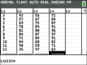
Step 1.
Enter the data into the lists.
For basic entry of data, see Basic
Commands.
The month numbers are in L1.
Syracuse temperatures are in L2.
Washington temperatures are in L3.
Austin temperatures are in L4. |
|
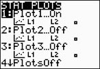
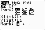
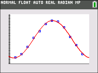
Step 2.
Create a scatter plot of the data.
Go to STATPLOT (2nd Y=)
and choose the first plot. Turn the plot
ON, set the icon to Scatter
Plot (the first one), set Xlist
to L1 and Ylist to
L2 (assuming that is where
you stored the data), and select a Mark of your choice. Zoom #9.
  |
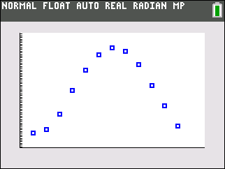
(Syracuse, NY) |
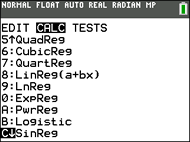
Step 3.
Choose the Sinusoidal Regression Model.
Press STAT, arrow right to
CALC, and arrow down to
C: SinReg. Hit
ENTER. When
SinReg appears on the home
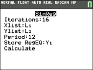
screen, type the parameters 16,
L1, L2, 12, Y1. The Y1
will put the equation into Y=
for you. (Y1 comes from VARS → YVARS, #Function, Y1 OR ALPHA F4)
PARAMETERS:
· SinReg(Iternations, Xlist, Ylist, Period, Store)
· In a sinusoidal regression, the "iterations" is the maximum number of times the SinReg command will iterate to find the equation. Any integer from1 to 16 can be used, but 16 generally gives a more accurate result than smaller integers. Default = 3.
Higher values may take more time to compute.
· The "period" is the horizontal distance between two maximums or two minimum points. If you leave the period empty, the calculator will take over.
· The "store" is the location where the equation will be stored. Default is Y1.
Notice that there is no correlation coefficient or coefficient of determination. |
(Syracuse, NY)
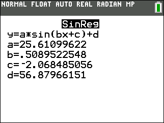
The sinusoidal regression equation is
y = 25.611 sin(0.509 x + (-2.068)) + 56.880 Be sure you notice when working with the calculator's sinusoidal equation, that the b has NOT been factored out. It is not the same as the equation
y = Asin(B(x - C)) + D. |
Step 4.
Graph the Sinusoidal Regression Equation from
Y1.
|
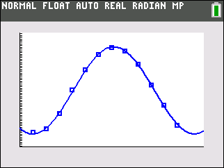
(Syracuse, NY) |
Step 5.
Get the sinusoidal equations for the other cities.
(Washington, DC)
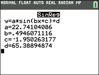
y = 22.741 sin(0.495x + (-1.950)) + 65.389
 |
(Austin, TX)
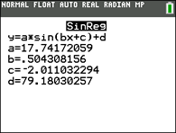
y = 17.742 sin(0.504x + (-2.011)) +79.180
|
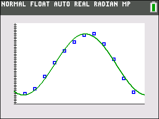
Step 6.
Graph all three cities on same grid.
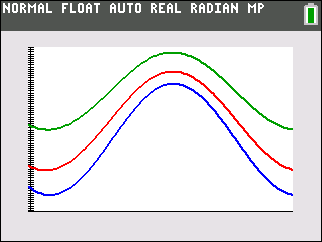 |
Do the graphs intersect? NO
Are these graphs representative of what was observed in the data? YES
Explain. If you examine the data, you notice that the cities are arranged such that Syracuse is "cold", Washington is "warm" and Austin is "hot" for every month. There will never be a point of intersection. |
|